Bias-Variance Tradeoff Simulation

When building machine learning models, we often try to estimate the real data as well as possible without overfitting or underfitting. One way of evaluating the accuracy of a model is by examining the Mean Squared Error (MSE): the mean squared distance between a predicted value and an observed value. MSE can be calculated for both training data and testing data; however, the training MSE typically isn’t helpful as it always decreases when the model fits the data better, regardless of overfitting. Testing MSE is usually a better indication of a model’s viability, especially when the testing set contains observations dissimilar to the training set. A relatively low testing MSE means that the model is a decent approximation of the true data.

From a theoretical approach, the expected MSE is defined as:

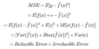
The bias and variance of a model are considered to be reducible error, meaning that they can be reduced by choosing a more optimal model. To find the most optimal model, we want to find the minimum sum between bias and variance.

What are Bias and Variance and why is there a tradeoff?

In this context, bias refers to how well a model matches the data whereas variance refers to how much a model is influenced by its training set. Let’s compare a linear model and a 10th-degree polynomial to illustrate the tradeoff between bias and variance. A linear model estimates two parameters (the intercept and slope of a line), whereas a 10th-degree polynomial model estimates eleven parameters (the intercept and ten coefficients for x^1 through x^10). Since a 10th-degree polynomial has 11 different parameters, it can take many different shapes depending on the training data, meaning that it is quite variable. However, the high flexibility allows the model to fit the training data really well, meaning that it has a low bias. On the other hand, a linear model has a high bias because it does not fit the data as well, but it has a low variance as its parameters won’t change as drastically in response to different training samples. A model can only have both a small bias and a small variance is if it is incredibly close to the actual distribution of data; otherwise, the bias and variance will trend in opposite directions.

Notice how the 10th-degree polynomial (green line) fits the data very well, but it varies greatly with a different sample. The linear model (light blue line) doesn’t fit the data as well, but it is certainly less variable.

Simulation

In order to further investigate the bias-variance tradeoff, I performed a simulation (click here to view GitHub repository) showing the test MSE for a linear, quadratic, cubic, and quintic model each trying to estimate a simple function:

f(x) = 2x + 5x^2 + E ; E ~ N(2, 5^2).

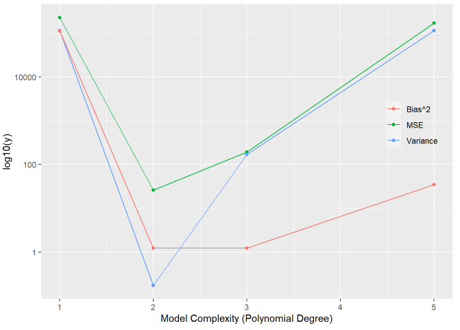
The simulation confirmed that a quadratic model was the best approximation of the true function. This isn’t a groundbreaking revelation though, we specifically knew that the underlying data was generated from a quadratic equation! Even though this is a greatly simplified example of a bias-variance decomposition, we can still generalize the concept to more complex data. In reality, we often don’t know the true underlying distribution of data, but using the mean squared error is one tool to show the utility of a machine learning model.