Image Compression (SVD, PCA, JPEG, and PNG)
The latter half of the “Advanced Predictive Models” course in my graduate program involved the meticulous discussion of matrix properties such as singular values, eigenvalues, and covariance structures in the context of data compression and dimensionality reduction. Many motivating examples involved performing compression techniques on digital images represented by matrices of pixel data. The motivations of data compression are intuitive in this setting: a single 4K resolution image can occupy up to 600 MB of storage space - with a surprising amount of redundant data. In class, we used SVD, PCA, and non-negative matrix factorization to process images, and the examples prompted me to research the intricacies of more popular and practical image compression algorithms like JPEG and PNG. SVD and PCA have more functional data science applications outside of image compression, but understanding how they work still provides some interesting analogs to niche compression methods such as JPEG and PNG.
Note: In this post, I discuss the intuition of each of these methods. For a comprehensive mathematical explanation and a Python implementation of these methods, check out the Jupyter Notebook I made to supplement this post on my GitHub.
Singular Value Decomposition (SVD)
SVD states that any matrix can be factorized as a linear combination of its left singular vectors (U), singular values (Σ), and the transpose of its right singular vectors (V transpose), where the singular values and singular vectors can essentially be interpreted as the magnitudes and directions of variance in the data.
This factorization is typically written such that the singular values are ordered in decreasing magnitude, meaning that the most important information in the matrix can be extrapolated from the first few singular values and vectors. This means it is possible to calculate a low-rank approximation of the factorized matrix to compress the image. The rank of a matrix refers to the number of linearly independent row or column vectors, so a low-rank approximation of a matrix is computed by using only a few linearly independent components (U and V transpose are the linearly independent components). Since a digital image can be written as a matrix, we can easily use SVD to calculate a low-rank approximation of an image, which should require less storage space.
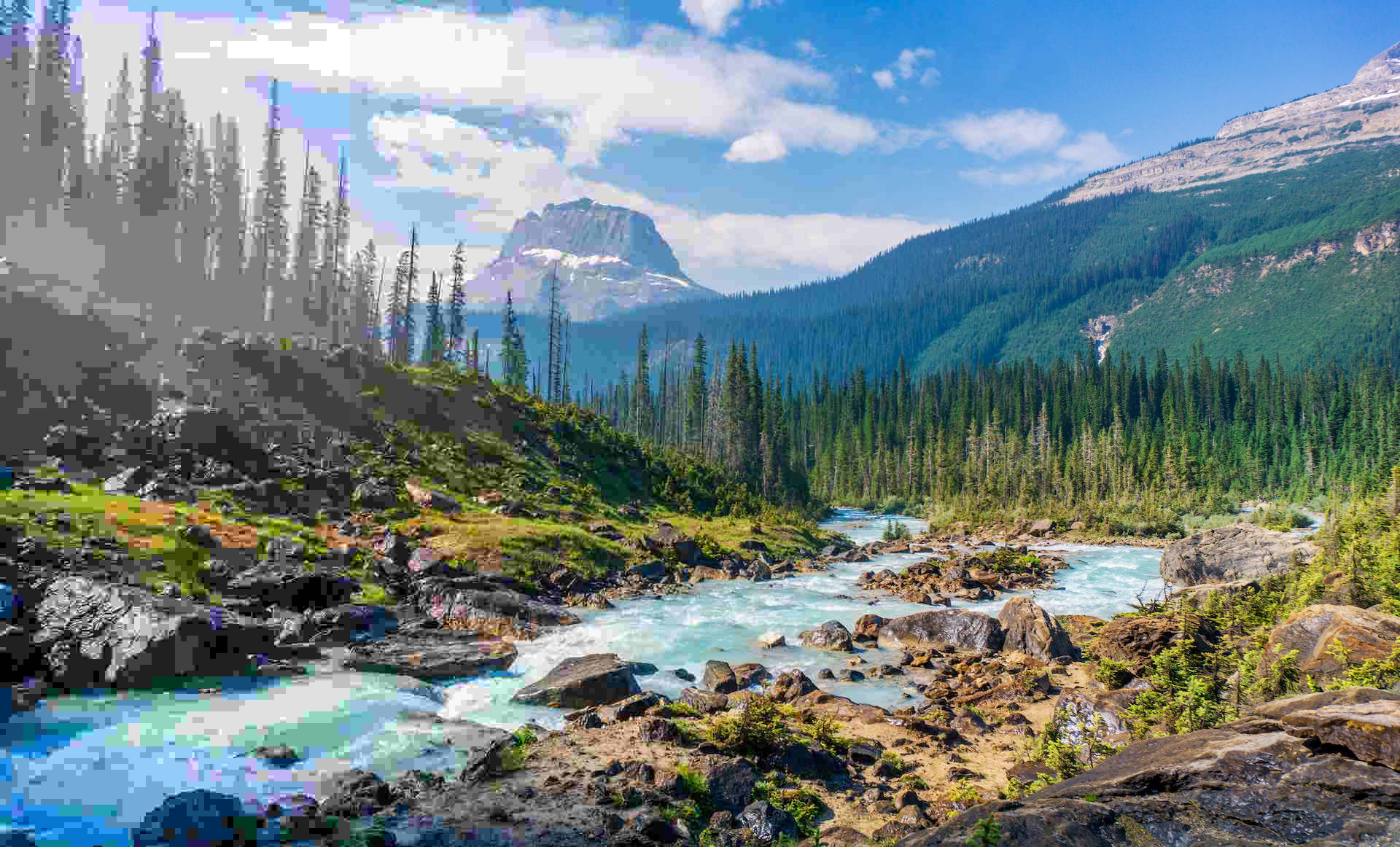
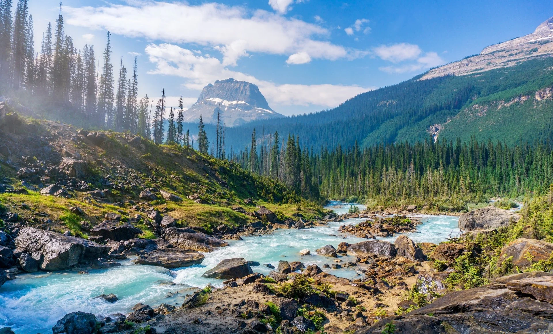
Here are some images that are compressed using SVD rank-k approximations:

Principal Component Analysis (PCA)
PCA is a dimensionality reduction technique frequently used on large datasets with many features per observation. It can reduce dimensionality by identifying the magnitudes and directions of the maximum variation in the data - known as calculating the top principal components. It uses the top principal components to linearly transform the data into a new coordinate system where the variation can be represented in fewer dimensions. Under certain circumstances, SVD and PCA are equivalent - I discuss when and why more thoroughly in the supplemental Jupyter Notebook.
PCA is commonly used to exclude redundant information and help identify trends or features across many images. Image datasets are a natural candidate for PCA because they typically have incredibly high dimensions. For example, a collection of 1000 images, each with a resolution of only 64 by 64 pixels, will result in a dataset that is 1000 rows and 4096 columns.
Using a Pokemon Image dataset, I recreated an image of a Pokemon with the top 100 principal components. PCA has more practical use cases in image processing, like identifying features of handwritten digits or facial recognition, but I figured that using Pokemon would be a more fun demonstration.

SVD and PCA have their respective use cases in the context of image processing and compression but are impractical options for reducing file size. Huge media files like raw images can seriously bottleneck the performance and loading times of web pages, so let’s take a look at JPEG and PNG: two of the most popular image compression file formats.
JPEG
JPEG is a lossy image compression algorithm and file format that finds a balance between retaining image quality and reducing file size. “Lossy” means that the algorithm will discard unimportant information in the image to make the file size smaller. In that respect, it is similar to SVD and PCA, although JPEG is computationally more efficient and directly compresses the file.
The JPEG algorithm utilizes matrix transformations, encoding techniques, and some clever tricks that take advantage of how our vision works. There are several variations that have subtle differences, but these are the general steps that the JPEG algorithm follows:
Convert the image from the conventional RGB color space to the YCrCb color space. This transforms the image from red, green, and blue color channels into a brightness channel and two alternative color channels before performing any type of compression. This is done because the human eye is more receptive to brightness rather than color, so isolating these channels helps prepare the image for the next steps.
Chroma downsampling or chroma subsampling. This step takes blocks of adjacent pixels in an image and averages or samples their two YCrCb color channels into one value per block per channel. This is a lossy step as it loses specific color information from individual pixels, but the difference is nearly imperceptible.
Discrete Cosine Transform (DCT). This step expresses each channel of the image as a weighted sum of different frequencies in preparation for the quantization step - this is a lossless step.
Quantization. Next, divide the coefficients obtained from the DCT by the corresponding elements of a quantization matrix, which is a grid that describes frequencies. Ideally, many of the resulting values of this operation will be zero, meaning that this representation of our image contains frequencies that our eyes won’t perceive and can be thrown away; this is where a lot of data can be truncated.
Entropy Encoding. Lastly, we want to encode the values from the quantization step in a way that can optimize storage. First, run-length encoding is performed to arrange the values that need to be stored, and then Huffman coding is performed to compress these values. Both of these encoding steps are lossless.
The image is stored in this encoded state as a .jpg file, meaning that JPEGs are actually not stored as an intelligible image; they are stored as a series of encoded values. Once an image is ready to be rendered or viewed, the JPEG algorithm is performed in reverse: undoing the encoding steps, quantization, and DCT, upscaling, and transforming the image back into the RGB color space. The algorithm drastically transforms the image to store it as a much smaller file, but the differences between the original image and its JPEG-compressed counterpart are usually unnoticeable.
PNG
In contrast to JPEG, PNG is a lossless algorithm, meaning that the original image’s quality is perfectly preserved after it is compressed. This makes PNGs more effective for capturing screenshots and detailed, high-frequency images.
Lossless algorithms have the strict constraint of not truncating any data, so they need to find a clever way to rewrite the original data to optimize byte usage. Here is the PNG algorithm’s approach:
Filtering. In the context of PNG, filtering refers to row-by-row operations that measure the differences between pixels. PNG defines five types of filters: None, Sub, Up, Average, and Paeth. Filtering transforms the pixel values so the upcoming encoding steps are more effective.
LZ77 Encoding. This compression algorithm optimizes storage space by referencing earlier instances of repetitive data. For example, if an image contains ten identical white pixels in a row, an LZ77 encoder will copy the first instance of the pixel to memory, then instead of storing the values of the next nine pixels, it instead stores nine references to the first pixel. The algorithm is capable of encoding much more complex patterns of repetitive data, but this trivial example still provides the fundamental intuition.
Huffman Coding. Just like the JPEG algorithm, the final compression step is Huffman coding. This lossless method is used to further optimize the storage of the LZ77 encoding. The combination of LZ77 Endcoding and Huffman coding is known as DEFLATE.
Fun fact: DEFLATE is also used in the ZIP algorithm, which is used to compress files to a .zip format.
The PNG algorithm stores the encoded image as a .png file, which like a JPEG, has to be decoded before being rendered or viewed. Although PNG only consists of filtering, LZ77, and Huffman coding, the algorithm is computationally expensive and relatively slow; however, the resulting file is still noticeably smaller than the original.
The details of the PNG algorithm are very complex and can be confusing without compartmentalized examples. Reducible has an excellent video with visual explanations of filtering, LZSS encoding, and Huffman encoding.
The differences between SVD, PCA, JPEG, and PNG provide incredible insight into how a similar problem can be approached with different solutions. Although SVD and PCA were formulated for purposes other than image compression, they still use a framework that can recreate an image by ignoring the least important aspects. JPEG and PNG are niche solutions that accomplish their job quite well - they have been around since the 90s and are still the most popular image compression algorithms. Further immersing myself in these processes has demonstrated the value of approaching problems from different perspectives and shows the ubiquity and versatility of problem-solving and data science.
Resources:
SVD and PCA
https://en.wikipedia.org/wiki/Singular_value
https://mse.redwoods.edu/darnold/math45/laproj/fall2005/ninabeth/FinalPresentation.pdf
https://en.wikipedia.org/wiki/Principal_component_analysis
https://en.wikipedia.org/wiki/Eigendecomposition_of_a_matrix
JPEG and PNG
https://www.youtube.com/watch?v=0me3guauqOU
https://www.youtube.com/watch?v=Kv1Hiv3ox8I
https://medium.com/@duhroach/how-png-works-f1174e3cc7b7