How Linear Regression Works
Linear regression is one of the first machine learning algorithms that many people study because of its intuitive, straightforward concept. However, its simplicity may lead some to overlook the math that enables the algorithm to plainly describe the relationship between variables. A deep understanding of the math and motivations behind linear regression is extremely valuable: Many other machine learning algorithms use surprisingly similar concepts. After reading this - regardless of your previous knowledge of machine learning - you will have a strong foundation about what linear regression is, how it works, and the pros and cons of using it.
Madis Lemsalu has a fantastic, brief video showing a graphical interpretation of regression and residuals.
The primary goals of linear regression are to approximate an unknown linear function and gain insight into how predictors affect a response. In a linear equation (y = ax + b), we already know the slope and intercept, so for any value of x, we can immediately determine the value of y. Linear regression uses data points to reverse engineer that dynamic: we already know x and y, so we try to estimate the values of a and b. In real data, however, predictors rarely correspond perfectly with the response, so linear regression models include a term called random error to account for the variation between x and y that cannot be predicted or explained. The differences between the actual values of y and the model’s predicted values of y are called residuals and are the key to approximating the aforementioned unknown function. Ideally, we want to find a slope and intercept, which I’ll refer to as parameters going forward, that makes the residuals as small as possible.
The full least squares derivation can be found on my GitHub.
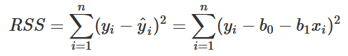
There are several different ways to calculate optimal parameters, but I’ll describe the method of least squares as it is quite popular and does a great job illustrating the fundamental motivations and math behind linear regression. Least squares refers to the process of minimizing the total sum of squared residuals; and almost every time something needs to be minimized or maximized in the context of machine learning, some form of calculus is involved. The derivation of least squares is not the most complex math you’ll see, but there is still some tricky, yet clever algebra used to estimate parameters. I included this derivation, along with a few examples on my GitHub for those interested - if not, just know that if the predicted values of y are consistently close to the actual values of y, the residuals are relatively small and the estimated parameters fit the data well.
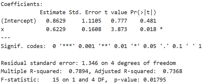
Output of a simple linear regression model performed in R. In this case, as x increases by 1 unit, y is expected to increase by .6229 units, and when x equals 0, y is expected to equal .8629.
Linear regression is incredibly useful because of its interpretability. Say that your least squares estimates for slope and intercept are 2 and 3, respectively. In the case of simple linear regression (SLR), where there is one predictor (x) and one response (y), a slope of 2 means that as x increases by 1 unit, y is expected to increase by 2 units and when x equals 0, y is expected to equal 3 - pretty straightforward.
Simple linear regression is great, but many machine learning problems seek to find relationships between a response and multiple predictors. What happens when you want to include more than one predictor in a model? Simple linear regression is no longer an option, but luckily the concepts discussed so far generalize into higher dimensions pretty well. Multiple linear regression is one solution: it extends the same concepts as SLR with just a small amount of extra complexity.
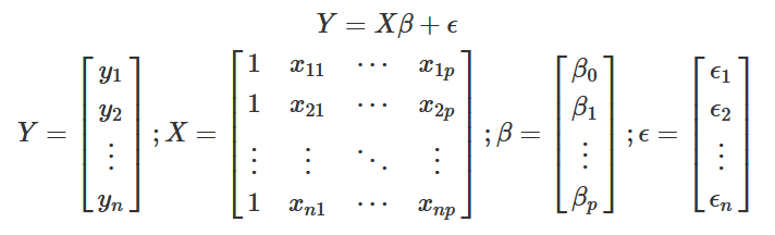
Linear regression model expressed with matrix notation
In general, least squares parameter estimation generates a system p+1 equations with p+1 unknown variables, where p is the number of predictors used for the regression. In SLR, you have 1 predictor, x, so there is a system of 2 equations with 2 unknowns, but multiple linear regression can create complex systems that may require some iterative processes to solve. Furthermore, a large number of predictors increases the chance of two or more predictors being correlated - meaning they provide similar information. This phenomenon, known as multicollinearity, can lead to incorrect coefficient estimates and may invalidate the model. A large number of variables also stretches the assumption that all of the predictors and the response are truly related by a linear equation. These are ultimately warnings rather than deterrents to using multiple linear regression: If all assumptions are satisfied and multicollinearity is not a concern, it is still one of the most effective and interpretable models.
Although I covered the essentials of linear regression, there are some details that I omitted for the sake of brevity and simplicity; entire books have been written to cover the theory and applications. If you want to learn more about linear regression, I suggest looking through the following resources:
A Refresher on Regression Analysis - Harvard Business Review: gives business applications for linear regression.
A Modern Approach to Regression with R: textbook that was used in my statistics-oriented Linear Regression course at Texas A&M. This was very helpful when I organized the most important components of regression.
How to implement Linear Regression from scratch with Python: YouTube video that walks through Linear Regression implementation in Python that provides a more technical overview that is applicable to many other forms of machine learning.